```{r setup}
#| include: false
# Load required packages
library(tidyverse)
library(knitr)
library(kableExtra)
# Format-aware table helper
fmt_kable <- function(data, align = NULL, bold_rows = NULL, highlight_row = NULL, ...) {
if (knitr::is_html_output()) {
tbl <- kable(data, align = align, ...)
tbl <- kable_styling(tbl, bootstrap_options = c("striped", "hover"))
if (!is.null(bold_rows)) tbl <- row_spec(tbl, bold_rows, bold = TRUE)
if (!is.null(highlight_row)) tbl <- row_spec(tbl, highlight_row, bold = TRUE, background = "#E8F5E9")
tbl
} else if (knitr::is_latex_output()) {
tbl <- kable(data, format = "latex", align = align, booktabs = TRUE, ...)
tbl <- kable_styling(tbl, latex_options = c("striped", "hold_position", "scale_down"))
if (!is.null(bold_rows)) tbl <- row_spec(tbl, bold_rows, bold = TRUE)
if (!is.null(highlight_row)) tbl <- row_spec(tbl, highlight_row, bold = TRUE)
tbl
} else {
kable(data, align = align, ...)
}
}
# Source manuscript functions
source("./R/manuscript_functions.R")
# Load data
omentum_full <- load_omentum_data("./data/omentum_recoded.csv")
micro_tracked <- read_csv("./data/microscopic_only_cases_analyzed.csv", show_col_types = FALSE)
# Compute statistics
cohort_stats <- get_cohort_stats(omentum_full)
grade_stats <- get_tumor_grade_stats(omentum_full)
metastasis_stats <- get_metastasis_distribution(omentum_full)
micro_stats <- get_microscopic_only_stats(omentum_full)
detection_stats <- get_first_detection_stats(micro_tracked)
# Bootstrap analysis
boot_results <- bootstrap_detection_probability(
micro_tracked$first_cassette_tumor_identified,
n_boot = 10000,
seed = 42
)
# Cumulative detection probabilities
cumulative_detection <- calculate_cumulative_detection(boot_results$q, max_cassettes = 10)
# Comparison by location
location_comparison <- compare_by_location(micro_tracked)
# Empirical proportion analysis
empirical_results <- calculate_empirical_detection(micro_tracked, max_cassettes = 10, n_boot = 10000, seed = 42)
empirical_stats <- calculate_empirical_probability(micro_tracked)
# Comparison of both methods
method_comparison <- compare_detection_methods(micro_tracked, max_cassettes = 10)
comparison_table <- create_method_comparison_table(method_comparison)
# Heterogeneity analysis
heterogeneity_results <- calculate_heterogeneity(micro_tracked)
# Stratified analysis by tumor burden
stratified_results <- stratify_by_tumor_burden(micro_tracked)
# Spatial clustering statistics
clustering_stats <- get_spatial_clustering_stats(micro_tracked)
# Beta-binomial sensitivity analysis
bb_results <- beta_binomial_sensitivity(
micro_tracked %>% filter(!is.na(NumberOfBlocksWithTumor)),
max_cassettes = 10
)
```
# Results
## Overall Cohort Characteristics
The mean age of the `r cohort_stats$n_total` patients was `r cohort_stats$age_mean` ± `r cohort_stats$age_sd` years (median: `r cohort_stats$age_median` years, IQR: `r cohort_stats$age_q25`-`r cohort_stats$age_q75` years). Primary tumor locations were distributed as follows: `r cohort_stats$n_endometrium` (`r cohort_stats$pct_endometrium`%) endometrial carcinomas, `r cohort_stats$n_ovary` (`r cohort_stats$pct_ovary`%) tubo-ovarian carcinomas, and `r cohort_stats$n_synchronous` (`r cohort_stats$pct_synchronous`%) synchronous tumors.
Regarding tumor grade classification, `r grade_stats$n_low_grade` (`r grade_stats$pct_low_grade`%) were low-grade tumors (grade 1 and 2 endometrioid carcinoma), `r grade_stats$n_high_grade` (`r grade_stats$pct_high_grade`%) were high-grade, and `r grade_stats$n_borderline` (`r grade_stats$pct_borderline`%) were serous borderline tumors.
```{r}
#| label: tbl-characteristics
#| tbl-cap: "Clinicopathologic Characteristics of the Study Cohort"
create_characteristics_table(omentum_full) %>%
fmt_kable(align = c("l", "r"), bold_rows = c(4, 8, 12))
```
The distribution of tumor grades across primary tumor locations is shown in @tbl-grade-by-location. Tubo-ovarian carcinomas were predominantly high-grade (`r round(100 * sum(omentum_full$TumorLocation == "Ovary" & omentum_full$TumorType == "High", na.rm = TRUE) / sum(omentum_full$TumorLocation == "Ovary", na.rm = TRUE), 1)`%), whereas endometrial carcinomas showed a more balanced distribution with `r round(100 * sum(omentum_full$TumorLocation == "Endometrium" & omentum_full$TumorType == "Low", na.rm = TRUE) / sum(omentum_full$TumorLocation == "Endometrium", na.rm = TRUE), 1)`% low-grade and `r round(100 * sum(omentum_full$TumorLocation == "Endometrium" & omentum_full$TumorType == "High", na.rm = TRUE) / sum(omentum_full$TumorLocation == "Endometrium", na.rm = TRUE), 1)`% high-grade tumors. All borderline tumors (n=`r grade_stats$n_borderline`) were of ovarian origin.
```{r}
#| label: tbl-grade-by-location
#| tbl-cap: "Distribution of Tumor Grade by Primary Tumor Location"
create_grade_by_location_table(omentum_full) %>%
fmt_kable(align = c("l", rep("c", 4)))
```
## Omental Metastasis Distribution
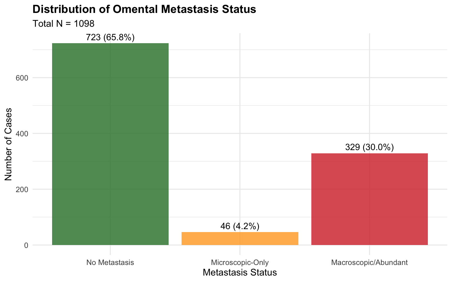
Of the `r cohort_stats$n_total` cases, `r metastasis_stats$n_no_tumor` (`r metastasis_stats$pct_no_tumor`%) showed no omental metastasis. `r metastasis_stats$n_macro` cases (`r metastasis_stats$pct_macro`%) had obvious/abundant macrometastasis. `r metastasis_stats$n_micro_only` cases (`r metastasis_stats$pct_micro_only`%) had micrometastasis detected.
```{r}
#| label: fig-metastasis-distribution
#| fig-cap: "Distribution of Omental Metastasis Status"
#| fig-width: 8
#| fig-height: 5
metastasis_data <- tibble(
Status = c("No Metastasis", "Microscopic-Only", "Macroscopic/Abundant"),
Count = c(metastasis_stats$n_no_tumor, metastasis_stats$n_micro_only, metastasis_stats$n_macro),
Percentage = c(metastasis_stats$pct_no_tumor, metastasis_stats$pct_micro_only, metastasis_stats$pct_macro)
) %>%
mutate(Status = factor(Status, levels = c("No Metastasis", "Microscopic-Only", "Macroscopic/Abundant")))
ggplot(metastasis_data, aes(x = Status, y = Count, fill = Status)) +
geom_bar(stat = "identity", alpha = 0.8) +
geom_text(aes(label = sprintf("%d (%.1f%%)", Count, Percentage)),
vjust = -0.5, size = 4) +
scale_fill_manual(values = c("#2E7D32", "#FFA726", "#D32F2F")) +
labs(
title = "Distribution of Omental Metastasis Status",
subtitle = sprintf("Total N = %d", cohort_stats$n_total),
x = "Metastasis Status",
y = "Number of Cases"
) +
theme_minimal(base_size = 12) +
theme(
legend.position = "none",
plot.title = element_text(face = "bold"),
axis.text.x = element_text(angle = 0, hjust = 0.5)
)
```
```{r}
#| include: false
# Compute metastasis-by-location inline values
n_macro_ovary <- sum(omentum_full$TumorLocation == "Ovary" & omentum_full$MacroscopicTumor == "Present", na.rm = TRUE)
n_macro_endo <- sum(omentum_full$TumorLocation == "Endometrium" & omentum_full$MacroscopicTumor == "Present", na.rm = TRUE)
n_micro_ovary_loc <- sum(omentum_full$TumorLocation == "Ovary" & omentum_full$MacroscopicTumor == "Absent" & omentum_full$MicroscopicTumor == "Present", na.rm = TRUE)
n_micro_endo_loc <- sum(omentum_full$TumorLocation == "Endometrium" & omentum_full$MacroscopicTumor == "Absent" & omentum_full$MicroscopicTumor == "Present", na.rm = TRUE)
```
The distribution of omental metastasis status by primary tumor location is shown in @tbl-metastasis-by-location. Macroscopic omental metastasis was markedly more common in tubo-ovarian carcinomas (`r round(100 * n_macro_ovary / cohort_stats$n_ovary, 1)`%) compared to endometrial carcinomas (`r round(100 * n_macro_endo / cohort_stats$n_endometrium, 1)`%). Microscopic-only metastasis was also more frequent in ovarian (`r round(100 * n_micro_ovary_loc / cohort_stats$n_ovary, 1)`%) than endometrial (`r round(100 * n_micro_endo_loc / cohort_stats$n_endometrium, 1)`%) carcinomas.
```{r}
#| label: tbl-metastasis-by-location
#| tbl-cap: "Distribution of Omental Metastasis Status by Primary Tumor Location"
create_metastasis_by_location_table(omentum_full) %>%
fmt_kable(align = c("l", rep("c", 4)))
```
## Microscopic-Only Metastasis Cases
Among the `r micro_stats$n_micro_total` patients with micrometastasis, the primary tumor locations were: `r micro_stats$n_micro_ovary` (`r micro_stats$pct_micro_ovary`%) ovarian and `r micro_stats$n_micro_endometrium` (`r micro_stats$pct_micro_endometrium`%) endometrial carcinomas. Regarding tumor morphology, `r micro_stats$n_micro_high_grade` (`r micro_stats$pct_micro_high_grade`%) were high-grade and `r micro_stats$n_micro_borderline` (`r micro_stats$pct_micro_borderline`%) were borderline. No low-grade tumors showed micrometastasis in this cohort.
## First Detection Analysis
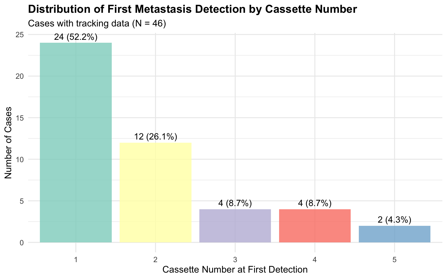
Among the `r micro_stats$n_micro_total` microscopic-only metastasis cases, `r detection_stats$n_with_tracking` (`r round(100 * detection_stats$n_with_tracking / micro_stats$n_micro_total, 1)`%) had complete tracking data regarding the cassette number in which metastasis was first detected. The mean cassette number at first metastasis detection was `r detection_stats$mean_first_detection` (median: `r detection_stats$median_first_detection`, SD: `r detection_stats$sd_first_detection`, range: `r detection_stats$range_min`-`r detection_stats$range_max`).
The distribution of first detection by cassette number was as follows: `r detection_stats$n_first_cassette` cases (`r detection_stats$pct_first_cassette`%) in the first cassette, and `r detection_stats$n_second_cassette` cases (`r detection_stats$pct_second_cassette`%) in the second cassette.
```{r}
#| label: tbl-first-detection
#| tbl-cap: "Distribution of First Detection by Cassette Number"
create_first_detection_table(micro_tracked) %>%
fmt_kable(align = c("c", "c", "c"))
```
```{r}
#| label: fig-first-detection
#| fig-cap: "Distribution of First Metastasis Detection by Cassette Number"
#| fig-width: 8
#| fig-height: 5
first_det_data <- create_first_detection_table(micro_tracked)
ggplot(first_det_data, aes(x = `Cassette Number`, y = `N Cases`, fill = `Cassette Number`)) +
geom_bar(stat = "identity", alpha = 0.8) +
geom_text(aes(label = sprintf("%d (%.1f%%)", `N Cases`, `Percentage (%)`)),
vjust = -0.5, size = 4) +
scale_fill_brewer(palette = "Set3") +
labs(
title = "Distribution of First Metastasis Detection by Cassette Number",
subtitle = sprintf("Cases with tracking data (N = %d)", detection_stats$n_with_tracking),
x = "Cassette Number at First Detection",
y = "Number of Cases"
) +
theme_minimal(base_size = 12) +
theme(
legend.position = "none",
plot.title = element_text(face = "bold")
)
```
## Detection Probability Analysis
We employed two complementary statistical approaches to estimate the per-cassette detection probability and ensure robustness of our sampling recommendations.
### Geometric Maximum Likelihood Estimation
The geometric MLE approach, estimated from the distribution of first detection cassette numbers, yielded a per-cassette detection probability of $q$ = `r boot_results$q` (95% CI: `r boot_results$ci_lower`-`r boot_results$ci_upper`). This corresponds to a `r boot_results$pct_q`% probability of detecting metastasis in any single cassette.
### Empirical Proportion Analysis
Across all `r detection_stats$n_with_tracking` cases, a total of `r empirical_stats$total_cassettes` cassettes were examined, of which `r empirical_stats$positive_cassettes` contained tumor. The empirical proportion yielded a detection probability of $q$ = `r empirical_stats$q` (`r empirical_stats$q_pct`%).
### Comparison of Methods
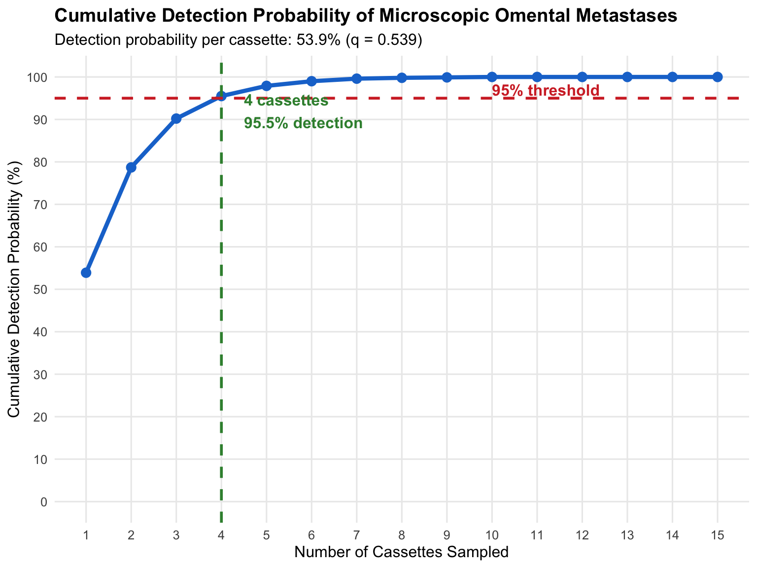
Both approaches converge on the same clinical recommendation, with 4 cassettes achieving >95% detection sensitivity (@tbl-method-comparison).
```{r}
#| label: tbl-method-comparison
#| tbl-cap: "Comparison of Detection Probability Estimates"
comparison_table %>%
fmt_kable(align = c("c", "c", "c", "c"), highlight_row = 4)
```
The geometric MLE provides a more conservative estimate (q = `r boot_results$q`), while the empirical proportion (q = `r empirical_stats$q`) incorporates information from all cassettes beyond first detection. **Both methods recommend sampling 4 cassettes** to achieve >95% detection: geometric MLE predicts `r cumulative_detection$cumulative_pct[4]`% and empirical proportion predicts `r empirical_results$cumulative_pct[4]`% cumulative detection with 4 cassettes.
```{r}
#| label: fig-cumulative
#| fig-cap: "Cumulative Detection Probability by Number of Cassettes Sampled"
#| fig-width: 8
#| fig-height: 6
cumulative_plot_data <- calculate_cumulative_detection(boot_results$q, max_cassettes = 15)
ggplot(cumulative_plot_data, aes(x = n_cassettes, y = cumulative_pct)) +
geom_line(color = "#1976D2", size = 1.5) +
geom_point(color = "#1976D2", size = 3) +
geom_hline(yintercept = 95, linetype = "dashed", color = "#D32F2F", size = 1) +
geom_vline(xintercept = 4, linetype = "dashed", color = "#388E3C", size = 1) +
annotate("text", x = 4.5, y = 92, label = sprintf("4 cassettes\n%.1f%% detection", cumulative_detection$cumulative_pct[4]),
hjust = 0, color = "#388E3C", fontface = "bold") +
annotate("text", x = 10, y = 97, label = "95% threshold",
hjust = 0, color = "#D32F2F", fontface = "bold") +
scale_x_continuous(breaks = 1:15) +
scale_y_continuous(breaks = seq(0, 100, 10), limits = c(0, 100)) +
labs(
title = "Cumulative Detection Probability of Microscopic Omental Metastases",
subtitle = sprintf("Detection probability per cassette: %.1f%% (q = %.3f)",
boot_results$pct_q, boot_results$q),
x = "Number of Cassettes Sampled",
y = "Cumulative Detection Probability (%)"
) +
theme_minimal(base_size = 12) +
theme(
plot.title = element_text(face = "bold"),
panel.grid.minor = element_blank()
)
```
## Heterogeneity and Extent of Omental Involvement
Assessment of heterogeneity across cases revealed a coefficient of variation (CV) of `r heterogeneity_results$cv` (`r heterogeneity_results$cv_pct`%), indicating `r tolower(heterogeneity_results$heterogeneity_level)` heterogeneity. Per-case positivity rates (proportion of cassettes with tumor) ranged from `r round(100*heterogeneity_results$min_rate, 1)`% to `r round(100*heterogeneity_results$max_rate, 1)`% (mean: `r round(100*heterogeneity_results$mean_rate, 1)`%, median: `r round(100*heterogeneity_results$median_rate, 1)`%).
Analysis of multi-block involvement revealed that `r clustering_stats$n_multiple_blocks` of `r clustering_stats$n_cases` cases (`r clustering_stats$pct_multiple_blocks`%) had tumor in multiple blocks, while only `r clustering_stats$n_single_block` cases (`r clustering_stats$pct_single_block`%) had tumor confined to a single block. The mean number of blocks containing tumor was `r clustering_stats$mean_blocks_with_tumor` per case. Since the spatial relationship between sampled blocks was not recorded, we cannot determine whether multi-block positivity reflects clustered or diffuse omental involvement. However, the high proportion of multi-block cases indicates that most microscopic metastases involve a sufficient volume of omental tissue to be detected across multiple independently sampled cassettes, which supports the validity of the per-cassette detection probability estimates.
## Beta-Binomial Sensitivity Analysis
As a sensitivity analysis accounting for inter-case heterogeneity in detection probability, we fitted a beta-binomial model to the per-case positivity rates. The estimated parameters were $\alpha$ = `r bb_results$alpha` and $\beta$ = `r bb_results$beta_param`, with an overdispersion parameter $\rho$ = `r bb_results$rho` (`r bb_results$rho_pct`%), confirming moderate heterogeneity. Under this model, the recommended 4 cassettes achieved `r bb_results$detection_at_4`% detection sensitivity, and 7 cassettes achieved `r bb_results$detection_at_7`% detection. The lower estimates compared to the geometric model (`r cumulative_detection$cumulative_pct[4]`% and `r cumulative_detection$cumulative_pct[7]`%, respectively) reflect the conservative nature of the beta-binomial approach, which accounts for the subset of cases with very focal disease and low per-cassette positivity. The geometric model estimates represent the average expected detection across all cases, which is the relevant metric for protocol development, while the beta-binomial highlights that cases with minimal tumor burden remain the most challenging to detect.
## Stratified Analysis by Tumor Burden
Cases were stratified based on the number of blocks containing tumor to assess heterogeneity in detection patterns (@tbl-stratified).
```{r}
#| label: tbl-stratified
#| tbl-cap: "Detection Characteristics Stratified by Tumor Burden"
stratified_results %>%
rename(
`Tumor Burden` = TumorBurden,
`N` = n,
`Mean First Detection` = mean_first_detection,
`Median First Detection` = median_first_detection,
`Detected at Cassette 1 (%)` = pct_detected_cassette_1,
`Detected by Cassette 2 (%)` = pct_detected_by_cassette_2,
`Detected by Cassette 4 (%)` = pct_detected_by_cassette_4
) %>%
fmt_kable(align = c("l", rep("c", 6)))
```
```{r}
#| include: false
# Extract stratified values for inline reporting
strat_high <- stratified_results %>% filter(TumorBurden == "High (4+ blocks)")
strat_low <- stratified_results %>% filter(TumorBurden == "Low (1 block)")
kw_stat <- attr(stratified_results, "kw_statistic")
kw_p_fmt <- attr(stratified_results, "kw_p_formatted")
kw_df <- attr(stratified_results, "kw_df")
```
Detection patterns differed significantly across tumor burden strata (Kruskal-Wallis H=`r kw_stat`, df=`r kw_df`, p=`r kw_p_fmt`). Cases with high tumor burden (4+ blocks involved) showed earlier detection (mean first cassette: `r strat_high$mean_first_detection`) compared to low burden cases with single block involvement (mean first cassette: `r strat_low$mean_first_detection`). Among low burden cases, only `r strat_low$pct_detected_cassette_1`% were detected at cassette 1, but `r strat_low$pct_detected_by_cassette_4`% were detected by cassette 4. This stratification demonstrates that the 4-cassette recommendation provides adequate sensitivity across the spectrum of tumor burden, being most critical for cases with focal disease.
## Comparison by Primary Tumor Site
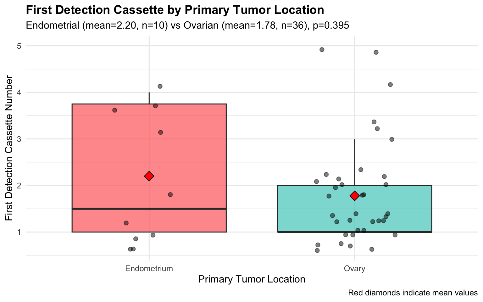
When examined by primary tumor site, the median first detection cassette for micrometastasis was `r location_comparison$median_endo` (mean `r location_comparison$mean_endo`) in endometrial cancers (n=`r location_comparison$n_endo`) and `r location_comparison$median_ovary` (mean `r location_comparison$mean_ovary`) in tubo-ovarian carcinomas (n=`r location_comparison$n_ovary`). This difference was not statistically significant (Mann-Whitney U test, p=`r location_comparison$wilcox_p_formatted`; mean difference `r location_comparison$mean_diff`, 95% CI: `r location_comparison$diff_ci_lower` to `r location_comparison$diff_ci_upper`; rank-biserial r=`r location_comparison$effect_size_r`).
```{r}
#| label: fig-location-comparison
#| fig-cap: "Comparison of First Detection Cassette by Primary Tumor Location"
#| fig-width: 8
#| fig-height: 5
comparison_data <- micro_tracked %>%
filter(TumorLocation %in% c("Endometrium", "Ovary"),
!is.na(first_cassette_tumor_identified))
ggplot(comparison_data, aes(x = TumorLocation, y = first_cassette_tumor_identified, fill = TumorLocation)) +
geom_boxplot(alpha = 0.7, outlier.shape = NA) +
geom_jitter(width = 0.2, alpha = 0.5, size = 2) +
stat_summary(fun = mean, geom = "point", shape = 23, size = 4, fill = "red") +
scale_fill_manual(values = c("#FF6B6B", "#4ECDC4")) +
labs(
title = "First Detection Cassette by Primary Tumor Location",
subtitle = sprintf("Endometrial (mean=%.2f, n=%d) vs Ovarian (mean=%.2f, n=%d), p=%s",
location_comparison$mean_endo, location_comparison$n_endo,
location_comparison$mean_ovary, location_comparison$n_ovary,
location_comparison$p_formatted),
x = "Primary Tumor Location",
y = "First Detection Cassette Number",
caption = "Red diamonds indicate mean values"
) +
theme_minimal(base_size = 12) +
theme(
legend.position = "none",
plot.title = element_text(face = "bold")
)
```
### Stratified Cumulative Detection by Primary Tumor Site
```{r}
#| include: false
# Stratified detection analysis by location
det_ovary <- subgroup_detection_analysis(
micro_tracked %>% filter(TumorLocation == "Ovary") %>% pull(first_cassette_tumor_identified)
)
det_endo <- subgroup_detection_analysis(
micro_tracked %>% filter(TumorLocation == "Endometrium") %>% pull(first_cassette_tumor_identified)
)
# Micrometastasis rates by grade in the full cohort
micro_by_grade <- get_micrometastasis_by_grade(omentum_full)
n_low_total <- micro_by_grade %>% filter(TumorType == "Low") %>% pull(n_total)
n_low_micro <- micro_by_grade %>% filter(TumorType == "Low") %>% pull(n_micro)
```
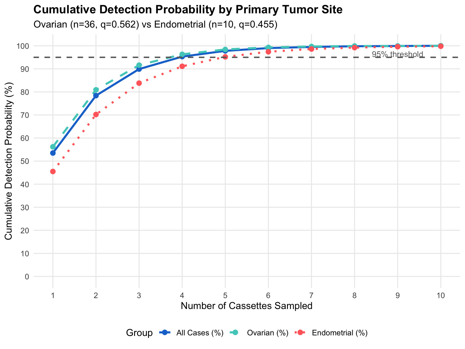
To evaluate whether sampling recommendations should differ by primary tumor site, we computed separate cumulative detection curves for ovarian and endometrial carcinomas (@tbl-detection-by-location; @fig-detection-by-location).
```{r}
#| label: tbl-detection-by-location
#| tbl-cap: "Cumulative Detection Probability by Primary Tumor Site"
create_location_detection_table(micro_tracked, max_cassettes = 10) %>%
fmt_kable(align = c("c", "c", "c", "c"), highlight_row = c(4, 5))
```
The per-cassette detection probability was higher for tubo-ovarian carcinomas (q=`r det_ovary$q`, 95% CI: `r det_ovary$ci_lower`-`r det_ovary$ci_upper`) than for endometrial carcinomas (q=`r det_endo$q`, 95% CI: `r det_endo$ci_lower`-`r det_endo$ci_upper`), though the confidence intervals overlap substantially. Ovarian carcinomas reached the 95% detection threshold at `r det_ovary$cassettes_for_95` cassettes, whereas endometrial carcinomas required `r det_endo$cassettes_for_95` cassettes. However, due to the small number of endometrial micrometastasis cases (n=`r det_endo$n`) and the wide, overlapping confidence intervals, this difference should be interpreted with caution and does not provide sufficient evidence to recommend different sampling protocols by primary tumor site at this time.
```{r}
#| label: fig-detection-by-location
#| fig-cap: "Cumulative Detection Probability by Primary Tumor Site"
#| fig-width: 8
#| fig-height: 6
plot_data <- create_location_detection_table(micro_tracked, max_cassettes = 10) %>%
pivot_longer(cols = -Cassettes, names_to = "Group", values_to = "Detection") %>%
mutate(Group = factor(Group, levels = c("All Cases (%)", "Ovarian (%)", "Endometrial (%)")))
ggplot(plot_data, aes(x = Cassettes, y = Detection, color = Group, linetype = Group)) +
geom_line(size = 1.2) +
geom_point(size = 2.5) +
geom_hline(yintercept = 95, linetype = "dashed", color = "grey40", size = 0.8) +
annotate("text", x = 9, y = 96.5, label = "95% threshold", color = "grey40", size = 3.5) +
scale_color_manual(values = c("All Cases (%)" = "#1976D2",
"Ovarian (%)" = "#4ECDC4",
"Endometrial (%)" = "#FF6B6B")) +
scale_linetype_manual(values = c("All Cases (%)" = "solid",
"Ovarian (%)" = "dashed",
"Endometrial (%)" = "dotted")) +
scale_x_continuous(breaks = 1:10) +
scale_y_continuous(breaks = seq(0, 100, 10), limits = c(0, 100)) +
labs(
title = "Cumulative Detection Probability by Primary Tumor Site",
subtitle = sprintf("Ovarian (n=%d, q=%.3f) vs Endometrial (n=%d, q=%.3f)",
det_ovary$n, det_ovary$q, det_endo$n, det_endo$q),
x = "Number of Cassettes Sampled",
y = "Cumulative Detection Probability (%)",
color = "Group",
linetype = "Group"
) +
theme_minimal(base_size = 12) +
theme(
plot.title = element_text(face = "bold"),
legend.position = "bottom",
panel.grid.minor = element_blank()
)
```
### Micrometastasis by Tumor Grade
Stratification of detection probability by tumor grade was not feasible because no low-grade tumors (0 of `r n_low_total`) exhibited microscopic omental metastasis in this cohort. All `r micro_stats$n_micro_total` microscopic-only cases were either high-grade (`r micro_stats$n_micro_high_grade`, `r micro_stats$pct_micro_high_grade`%) or borderline (`r micro_stats$n_micro_borderline`, `r micro_stats$pct_micro_borderline`%). The absence of micrometastasis in low-grade tumors, while not proving that it cannot occur, suggests that the clinical yield of extensive omental sampling in confirmed low-grade endometrioid carcinomas may be limited. This observation may have implications for risk-adapted sampling strategies, though it should be validated in larger studies specifically powered to detect low-frequency events in low-grade tumors.
```{r}
#| label: tbl-micro-by-grade
#| tbl-cap: "Incidence of Microscopic Omental Metastasis by Tumor Grade"
micro_by_grade %>%
rename(
`Tumor Grade` = TumorType,
`Total Cases` = n_total,
`Microscopic Metastasis` = n_micro,
`Incidence (%)` = pct_micro
) %>%
fmt_kable(align = c("l", "c", "c", "c"))
```